One-Dimensional Particle in a Box
The Particle in a Box (PIB) is the simplest of the quantum mechanical models we will see that can be solved exactly. It provides a scaffolding for understanding how quantum models are constructed and interpreted.
Creating the Model
We begin by simply drawing a box:
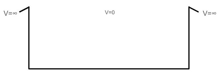
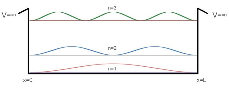
The first condition we impose on the box is that the potential energy, V, outside of the box is infinite and the potential energy inside of the box is zero; these can be thought of as walls of potential energy. We can represent this in our box:
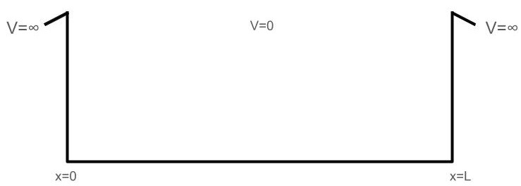
Next, we will define our box to be along the x-axis, such that the left wall is the position x=0 and the right wall is the position x=L; where L is the length of the box.
Now we will impose boundary conditions on our box. Boundary conditions, in this case, describe the behavior of a wavefunction at the two “boundaries” of the box. We have seen previously that the wavefunction describes the probability of finding the particle at a given position. Since we want our particle to be inside of the box, hence the name Particle in a Box, we impose the condition that there is no probability of finding the particle outside of the box. Also, we have seen the wavefunction must be differentiable to satisfy the Schrödinger Equation. Combining both of these requirements, we have the following boundary conditions:
\[\begin{align} \psi(x)|_{x=0}=0 \\ \psi(x)|_{x=L}=0 \end{align}\]The only wavefunction which satisfies these boundary conditions is of the form:
\[\begin{align} \psi(x)=A\sin(kx) \end{align}\]Where A is some arbitrary amplitude and k is the spatial frequency. The first boundary condition will be true for any value of k, but the second only allows for discrete values of k. Evaluating:
\[\begin{align} \psi(x)|_{x=L}=A&\sin(kl)=0 \\ \sin(kL)&=0 \\ kL=n\pi \hspace{0.5cm} & \hspace{0.5cm} n \in \mathbb{Z}^+ \\ k=\frac{n\pi}{L} \hspace{0.5cm} & \hspace{0.5cm} n \in \mathbb{Z}^+ \end{align}\]This is notably the most important result of the Particle in a Box exercise. Here we see that only discrete spatial frequencies, which “fit” inside of the box, are allowed. In quantum mechanics this is called quantization and, as we have seen here, it is a direct result of boundary conditions.
We can substitute the result for $k$ into our general PIB wavefunction:
\[\begin{align} \psi(x) & =A\sin(kx) \\ & =A\sin(\frac{n\pi x}{L}) \hspace{1cm} n \in \mathbb{Z}^+ \end{align}\]Since n is the variable which quantizes the wavefunction, we refer to it as a quantum number for this system.
Energy of the Particle
It was shown previously that the energy of a free particle is given by:
\[\begin{align} E=\frac{\hbar^{2}k^{2}}{2m} \end{align}\]Where is the reduced Planck’s constant, k is the spatial frequency of the wavefunction, and m is the mass of the particle. Substituting the PIB spatial frequency yields:
\[\begin{align} E_{n} & = \frac{\hbar^{2}(\frac{n\pi}{L})^{2}}{2m} \hspace{3cm}&n \in \mathbb{Z}^+\\ &= \frac{h^{2}n^{2}\pi^{2}}{(2\pi)^{2}(2m)(L^{2})} &n \in \mathbb{Z}^+\\ &= \frac{h^{2}n^{2}}{8mL^{2}} &n \in \mathbb{Z}^+ \end{align}\]Here the energy of the particle is proportional to the square of its quantum number, n. The mathematical significance of this can be seen by looking at the energy difference between two consecutive energy levels, \(n_{1}\) and \(n_{2}\):
\[\begin{align} \Delta E_{n_{2}-n_{1}} &=E_{n_{2}}-E_{n_{1}} \hspace{3cm}&n \in \mathbb{Z}^+ \hspace{5mm}&n_{2}>n_{1}\\ &= \frac{h^{2}n^{2}_{2}}{8mL^{2}} - \frac{h^{2}n^{2}_{1}}{8mL^{2}} &n \in \mathbb{Z}^+ \hspace{5mm}&n_{2}>n_{1}\\ &= \frac{h^{2}}{8mL^{2}}(n^{2}_{2}-n^{2}_{1}) &n \in \mathbb{Z}^+ \hspace{5mm}&n_{2}>n_{1} \end{align}\]So the difference between two consecutive energy levels increases with n. We can visualize this by co-plotting the first three energy levels’ respective wavefunctions and calculating their approximate energy differences inside of our box:
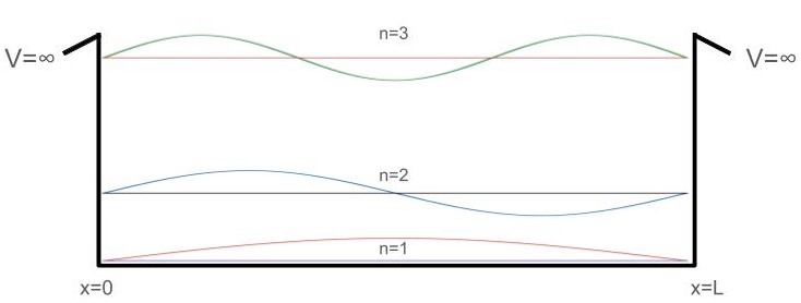
Co-plotting these wavefunctions also highlights an interesting property of PIB wavefunctions. For odd n’s, the wavefunctions are symmetric about \(\frac{L}{2}\). For even n’s, the wavefunctions are antisymmetric about \(\frac{L}{2}\).
Finally, we can look at the probability density of these first three wavefunctions by taking their square modulus:
Here we can clearly see the nodes of the wavefunction. A wavefunction’s node is a position where the wavefunction changes sign and its probability density is equal to zero at these points. We can also construct a formula to quickly find the number of nodes that a given PIB wavefunction will have:
\[number\ of\ nodes=n-1\]Normalizing the Wavefunction
Now looking back at our PIB wavefunction:
\[\psi(x)=A\sin(\frac{n\pi x}{L})\]There is still an unknown variable here; the amplitude of the wave, A. We will solve for this variable through the process of normalization. To normalize this wavefunction, we will make the statement that the area of the probability density is equal to one. This comes from the fact that there is only one particle that must be in the box at all times. So we now have the normalization condition:
\[\int_{0}^{L}|\psi(x)|^{2}dx=1\]Substituting our wavefunction:
\[\int_{0}^{L}[A\sin(\frac{n\pi x}{L})][A\sin(\frac{n\pi x}{L})]dx=1\]We will now introduce the variable N, for normalization constant, and set it equal to A. Substituting yields:
\[\int_{0}^{L}N^{2}\sin^{2}(\frac{n\pi x}{L})dx=1\]Since N is a constant and does not depend on x:
\[N^{2}\int_{0}^{L}\sin^{2}(\frac{n\pi x}{L})dx=1\]Using a table of integrals to solve:
\[N^{2}[\frac{x}{2}-\frac{\sin(\frac{2n\pi x}{L})}{4\frac{n\pi}{L}}]\bigg\rvert_{0}^{L}=1\]Evaluating:
\[N^{2}[\frac{L}{2}-0-0+0]=1\]Solving for N:
\[\begin{align} N^{2} &=\frac{2}{L} \\ N &=\sqrt{\frac{2}{L}} \end{align}\]Substituting this into the PIB wavefunction yields the solutions to the 1D PIB Schrödiner equation:
\[\psi(x)=\sqrt{\frac{2}{L}}\sin(\frac{n\pi x}{L}) \hspace{1cm} n \in \mathbb{Z}^{+}\]Page Author: Logan Grady