Second Law of Thermodynamics
Second Law of Thermodynamics
-
Rudolph Causius wrote in “The Mechanical Theory of Heat” (1879) that
The fundamental laws of the universe which correspond to the two fundamental theorems of the mechanical theory of heat:
- The energy of the universe is constant.
- The entropy of the universe tends to a maximum.
- The energy of the universe is constant.
The Second Law is Still Studied
In a 2010 interview, Sean M. Carroll from CalTech said
I’m trying to understand how time works. And that’s a huge question that has lots of different aspects to it. A lot of them go back to Einstein and spacetime and how we measure time using clocks. But the particular aspect of time that I’m interested in is the arrow of time: the fact that the past is different from the future. We remember the past but we don’t remember the future. There are irreversible processes. There are things that happen, like you turn an egg into an omelet, but you can’t turn an omelet into an egg.
Heat Engines and the Carnot Cycle
Sadi Carnot (1796-1832)
\(\;\)
A Heat Engine
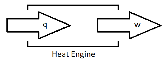
- Nature prevents the complete conversion of energy into work
-
Leads to an important statement of
The Second Law of Thermodynamics It is impossible to convert heat into an equivalent amount of work without some other changes occurring in the universe.
\(\;\)
A More Realistic Heat Engine
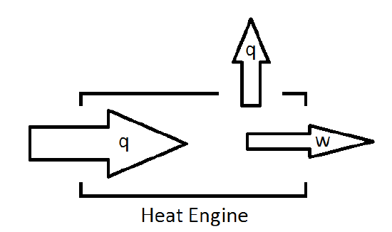
- The fraction of the heat provided to the engine to the amount of work the engine produces defines the efficiency of the engine.
\(\;\)
The Carnot Engine
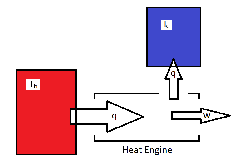
- A Carnot engine draws heat from a hot resevoir converts it to work and heat, the output heat is dumping into the cold resevoir.
The Carnot Cycle
- The Carnot Cycle is the cycle of steps that the engine undergoes in order to draw in heat and convert it to work in the Carnot engine.
-
The steps of the Carnot Cycle are:
- Isothermal expansion (\(dU=0\)) from \(P_1\) and \(V_1\) to \(P_2\) and \(V_2\) at \(T_h\) (temperature of the hot reservoir)
- Adiabatic expansion (\(q=0\)) from \(P_2,\, V_2,\, T_h\) to \(P_3,\,V_3,\,T_c\)
- Isothermal compression (\(dU=0\)) from \(P_3\) and \(V_3\) to \(P_4\) and \(V_4\) at \(T_c\) (temperature of the cold reservoir)
- Adiabatic compression (\(q=0\)) from \(P_4,\,V_4,\,T_c\) to \(P_1,\,V_1,\,T_h\)
\(\;\)
Plot of Carnot Cycle

Anaylsis of the Carnot Cycle
- The cycle is closed (ending state and initial state are equal)
- This means that any state function must have no net change
- The efficiency can be expressed as \[ \epsilon=\frac{w_{net}}{\left| q_h\right|}=\frac{|w_1|+\cdots +|w_n|}{|q_h|} \]
| Step | Heat | Work |
|---|---|---|
| 1 | \(q_h=-nRT_h\ln\left(\frac{V_2}{V_1}\right)\) | \(nRT_h\ln\left(\frac{V_2}{V_1}\right)\) |
| 2 | \(0\) | \(-C_V\left(T_c-T_h\right)\) |
| 3 | \(q_c=-nRT_c\ln\left(\frac{V_4}{V_3}\right)\) | \(nRT_c\ln\left(\frac{V_4}{V_3}\right)\) |
| 4 | \(0\) | \(C_V\left(T_h-T_c\right)\) |
\[ w_{tot} = nRT_h \ln \left(\frac{V_2}{V_1}\right) + nRT_c \ln \left(\frac{V_4}{V_3}\right) \]
\[ \epsilon = \frac{w_{tot}}{\left| q_h\right|} = \frac{nRT_h \ln \left(\frac{V_2}{V_1}\right) + nRT_c \ln \left(\frac{V_4}{V_3}\right)}{nRT_h\ln\left(\frac{V_2}{V_1}\right)} \]
Simplification
- When we studied the first law of thermodynamics we learned that \[ \left( \frac{V_2}{V_1} \right) = \left( \frac{T_2}{T_1} \right)^{-\frac{C_V}{R}} \Rightarrow \left( \frac{V_2}{V_1} \right) = \left( \frac{T_1}{T_2} \right)^{\frac{C_V}{R}} \]
- This means that \[ \text{Step 2: }\frac{V_3}{V_2} = \left(\frac{T_h}{T_c}\right)^\frac{C_V}{R} \;\;\text{ and }\;\; \text{Step 4: }\frac{V_1}{V_4} = \left(\frac{T_c}{T_h}\right)^\frac{C_V}{R} \] and step 4 can be rearranged to \[ \frac{V_4}{V_1} = \left(\frac{T_h}{T_c}\right)^\frac{C_V}{R} \]
- The right-hand side (RHS) of those equations are the same so we can equal their left-hand sides (LHS) \[ \frac{V_3}{V_2}=\frac{V_4}{V_1} \Rightarrow \frac{V_2}{V_1}=\frac{V_3}{V_4} \]
- Now we can simplify our efficiency equation \[ \begin{eqnarray} \epsilon &=& \frac{nRT_h \ln \left(\frac{V_2}{V_1}\right) + nRT_c \ln \left(\frac{V_4}{V_3}\right)}{nRT_h\ln\left(\frac{V_2}{V_1}\right)} \\ &=& \frac{nRT_h \ln \left(\frac{V_2}{V_1}\right) - nRT_c \ln \left(\frac{V_2}{V_1}\right)}{nRT_h\ln\left(\frac{V_2}{V_1}\right)} = \frac{T_h-T_c}{T_h}=\epsilon_{max} \end{eqnarray} \]
\(\;\)
Example 5.1
What is the maximum efficiency of a freezer set to keep ice cream at a cool \(-10^\circ C\), which it is operating in a room that is \(25^\circ C\)? What is the minimum amount of energy needed to remove \(1.0 J\) from the freezer and dissipate it into the room?
Entropy
Total Heat Transfered
- In the Carnot cycle the total heat transfered is \[ q_{tot}=nRT_h\ln\left(\frac{V_2}{V_1}\right)+nRT_c\ln\left(\frac{V_4}{V_3}\right) \]
- Using our volume relationship we found earlier that \(\frac{V_2}{V_1}=\frac{V_3}{V_4}\) \[ q_{tot}=nRT_h\ln\left(\frac{V_2}{V_1}\right)-nRT_c\ln\left(\frac{V_2}{V_1}\right) \]
\(\;\)
Analysis of Total Heat Transfered
\[ q_{tot}=nRT_h\ln\left(\frac{V_2}{V_1}\right)-nRT_c\ln\left(\frac{V_2}{V_1}\right) \]
- This is a cyclic process so state variables must have zero total change
- The total heat transfered, however, will only be zero if \(T_h=T_c\) which makes no sense
- This means that heat, \(q\), is not a state variable
- If temperature is the problem, what if we divide it away? \[ \sum_i \frac{q_i}{T_i} = \frac{nRT_h\ln\left(\frac{V_2}{V_1}\right)}{T_h} - \frac{nRT_c\ln\left(\frac{V_2}{V_1}\right)}{T_c}=0 \]
\(\;\)
A New State Function - Entropy
\[ \sum_i \frac{q_i}{T_i} = \frac{nRT_h\ln\left(\frac{V_2}{V_1}\right)}{T_h} - \frac{nRT_c\ln\left(\frac{V_2}{V_1}\right)}{T_c}=0 \]
- The sum shows that the ratio of heat to temperature change is a state function
- This leads to our definition of entropy, a state function \[ dS \equiv \frac{dq_{rev}}{T} \]
- In general, \(dq_{rev}>dq\) since the reversible pathway defines the maximum heat flow
Calculating Entropy Changes
Isothermal Changes
Consider an isothermal expansion of an ideal gas from \(V_1\) to \(V_2\) \[ \begin{eqnarray} dq &=& \frac{nRT}{V}dV \\ \frac{dq}{T} &=& nR\frac{dV}{V} \\ \Delta S = \int \frac{dq}{T} &=& nR\int_{V_1}^{V_2} \frac{dV}{V} = nR\ln \left(\frac{V_2}{V_1}\right) \end{eqnarray} \]
\(\;\)
Example 5.2
Calculate the entropy change for \(1.00 mol\) of an ideal gas expanding isothermally from a volume of \(24.4 L\) to \(48.8 L\).
\(\;\)
Isobaric Changes
For isobaric changes \[ dq=nC_P\,dT \] so \[ \begin{eqnarray} \frac{dq}{T} &=& nC_P\frac{dT}{T} \\ \Delta S = \int \frac{dq}{T} &=& nC_P \int_{T_1}^{T_2} \frac{dT}{T} = nC_P\ln \left(\frac{T_2}{T_1}\right) \end{eqnarray} \] If instead, \(C_P = a+bT+\frac{c}{T_2}\) then \[ \Delta S = n \left[ a\ln\left(\frac{T_2}{T_1}\right) + b\left(T_2-T_1\right) +\frac{c}{3}\left(\frac{1}{T_2^4}-\frac{1}{T_1^4}\right) \right] \]
\(\;\)
Isochoric Changes
For isochoric changes \[ dq=nC_V\,dT \] so \[ \begin{eqnarray} \frac{dq}{T} &=& nC_V\frac{dT}{T} \\ \Delta S = \int \frac{dq}{T} &=& nC_V \int_{T_1}^{T_2} \frac{dT}{T} \\ \Delta S &=& nC_V \ln \left(\frac{T_2}{T_1}\right) \end{eqnarray} \]
\(\;\)
Adiabatic Changes
- In adiabatic changes \(dq=0\). Therefore, in adiabatic changes \[ dS=\frac{dq}{T}=0 \]
- We often refer to adiabatic processes as isentropic
\(\;\)
Phase Changes
- We experience a lot of phase changes in chemistry
- The common phase changes that we experience occur open to our atmosphere
- Being open to the atmosphere means that it is isobaric
- We can calculate the change in entropy as \[ \Delta S = \frac{q}{T}=\frac{\Delta H_{phase}}{T} \]
\(\;\)
Example 5.3
The enthalpy of fusion for water is \(6.01 \frac{kJ}{mol}\). Calculate the entropy change for \(1.0 mole\) of ice melting to form liquid at \(273 K\).
Comparing the System and the Surroundings
Example 5.4
Consider \(18.02 g\) (\(1.00 mol\)) of ice melting at \(273 K\) in a room that is \(298 K\). Calculate \(\Delta S\) for the ice, the surrounding room, and of the universe. (\(\Delta H_{fus} = 6.01 \frac{kJ}{mol}\))
\(\;\)
Example 5.5
A \(10.0 g\) piece of metal (\(C = 0.250 \frac{J}{g\,^\circ C}\)) initially at \(95^\circ C\) is placed in \(25.0 g\) of water initially at \(15^\circ C\) in an insulated container. Calculate the final temperature of the metal and water once the system has reached thermal equilibrium. Also, calculate the entropy change for the metal, the water, and the entire system.
A New Way to State the 2nd Law
- We know that \[ \Delta S_{univ} = \Delta S_{sys} + \Delta S_{surr} \]
-
We can therefore state the second law as
The entropy of the universe increases in any spontaneous change.
- The “direction of spontaneous” is the natural direction of change
- This means that entropy is tied to the natural direction of the flow of time
Clausius Inequality
- The second law can be summed up in simple mathematical expression called the Clausius Inequality \[ \Delta S_{sys} \le 0 \] which must be true for any spontaneous process
- We can also write this as \[ \oint \frac{dq}{T} \le 0 \]
Entropy and Disorder
\(\;\)
Example 5.6
Calculate the entropy of a carbon monoxide crystal, containing \(1.00 mol\) of \({CO}\), and assuming that the molecules are randomly oriented in one of two equivalent orientations.