Eigenfunction for a Quantum Harmonic Oscillator
In this section, we will state and discuss the solution of the wave function for the quantum harmonic oscillator. Afterward, we will prove that the solution’s eigenvalue \(E\) is consistent with the well-known and established energy values of the system, thereby proving the solutions’ validity. We will begin by declaring Schrodinger’s equation.
Schrodinger Equation for a Quantum Harmonic Oscillator
Mentioned previously in the Harmonic Oscillator section 1, Schrodinger’s equation for a quantum harmonic oscillator is \(H\psi + V\psi= E\psi\), where \(H=\) \(\frac{-ℏ^2}{2m} ∇^2\), \(V=\) \(\frac{1}{2}kx^2\), and \(\psi\) is the particle’s wave function. Note \(V\) is the potential energy function of a harmonic oscillator.
Thus, with these definitions included, Schrodinger’s equation is
\[\frac{-ℏ^2}{2m} ∇^2\psi + \frac{1}{2}kx^2\psi= E\psi\]Definition and Discussion of the Eigenfunction for Harmonic Oscillator
It has been determined that the energies permitted by the boundary conditions for Schrodinger’s equation for an oscillator are \(E_v = (v + \frac{1}{2})ℏ\omega\) 1, where \(\omega=\sqrt{\frac{k_f}{m}}\). We will later use this fact to prove that the precise solution to Schrodinger’s Equation for a quantum harmonic oscillator is
\[\psi_v(y) = N_vH_v(y)e^\frac{-y^2}{2}\]where \(y = \frac{x}{\alpha}\), \(\alpha = (\frac{ℏ^2}{mk_f})^\frac{1}{4}\), and \(N_v\) is the normalization constant \(N_v =\frac{1}{\alpha\pi^\frac{1}{2}2^vv!}\)
There are several oddities in this solution that distinguish it from the previously discussed wave functions, specifically with the terms \(H_v\) and \(e^\frac{-y^2}{2}.\) The exact development of this model will not be discussed, but we can comment on the significance of these terms. The term \(e^\frac{-y^2}{2}\) represents the Gaussian curve, reflecting the probabilistic nature to the solution of the equation. Whereas \(H_v\), known as the Hermite polynomials, are a sequence of polynomials with its expression depending on frequency \(v\), shown in the table below: 2
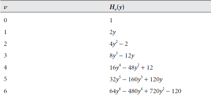
For each \(v\), the highest value exponent of \(y\) at each level of \(H_v\) is equal to frequency \(v\). The order of \(H_v\) determines the symmetry of the solution, which is valuable in charcaterizing the particle’s properties. The image below displays the solutions to \(\psi_v(y) = N_vH_v(y)e^\frac{-y^2}{2}\) with discretely increasing \(v\). 2
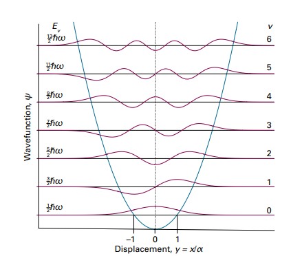
Plotted along with the solutions is the potential energy curve (blue parabola). The wave functions corresponding to even \(v\) are symmetric with respect to \(y=0\) and those corresponding to odd \(v\) are antisymmetric with respect to \(y=0\). As x approaches 0, the Gaussian function approaches 1, and so \(H_v\) dominates the behavior of the wave funtion. However, as x approaches infinity, the dampening effect of the Gaussian funtion dominates \(H_v\), forcing the function to approach zero.
Proof of the Solution by Evaluating Eigenvalue E
To verify that the solutions are correct we will evaluate the solution at ground state (\(v=0\)). Afterwards, we can determine the eigenvalue \(E_0\) and evaluate its consistency with the expected energy level for a quantum harmon oscillator \(E_v = (v + \frac{1}{2})ℏ\omega\).
The solution at ground state, \(v=0\), is
\[\psi_0(y) = N_0H_0(y)e^\frac{-y^2}{2}\]Using the \(H_v\) table above, we find that at \(v=0\), \(H_0 = 1\). We then substitute \(H_0 = 1\) and the constant \(y = \frac{x}{\alpha}\) into the solution to get
\[\psi_0(x) = N_0e^\frac{-x^2}{2\alpha^2}\]To apply the solution to the Hamiltonian of Schrodinger’s equation, we need the expression for \(\frac{d^2}{dx^2}\psi_0(x)\). To obtain it, we must first compute \(\frac{d}{dx}\psi_0(x)\) as follows:
\[\frac{d}{dx}\psi_0(x) = \frac{d}{dx}(N_0e^\frac{-x^2}{2\alpha^2}) = -N_0(\frac{x}{\alpha^2})e^\frac{-x^2}{2\alpha^2}\]We then take the derivative of the above result by employing the product rule:
\[-\frac{d}{dx}N_0(\frac{x}{\alpha^2})e^\frac{-x^2}{2\alpha^2} = -[(\frac{d}{dx}N_0\frac{x}{\alpha^2})e^\frac{-x^2}{2\alpha^2} + N_0\frac{x}{\alpha^2}(\frac{d}{dx}e^\frac{-x^2}{2\alpha^2})]\]Which evaluates to:
\[=-\frac{N_0}{\alpha^2}e^\frac{-x^2}{2\alpha^2} + N_0(\frac{x}{\alpha^2})^2e^\frac{-x^2}{2\alpha^2}\]Upon substituting \(\psi_0\) = \(N_0(x)e^\frac{-x^2}{2\alpha^2}\), we arrive at the final result:
\[\frac{d^2}{dx^2}\psi_0(x) = \frac{x^2}{\alpha^4}\psi_0 - \frac{1}{\alpha^2}\psi_0\]As the formula for \(\frac{d^2}{dx^2}\psi_0(x)\) is now known, we can substitute it into Schrodinger’s equation to obtain
\[\frac{-ℏ^2}{2m} (\frac{x^2}{\alpha^4}\psi_0 - \frac{1}{\alpha^2}\psi_0) + \frac{1}{2}kx^2\psi_0= E_0\psi_0\]After substituting \(\alpha = (\frac{ℏ^2}{mk_f})^\frac{1}{4}\) into the above expression and simplifying it, we receive
\[\frac{1}{2}\sqrt{\frac{k_f}{m}}ℏ\psi_0 = E_0\psi_0\]And finally, substituting \(\omega=\sqrt{\frac{k_f}{m}}\) provides us with our final result:
\[\frac{1}{2}ℏ\omega\psi_0 = E_0\psi_0\]As we can see, the eigenvalue, \(E_0\), is
\[E_0 = \frac{1}{2} \hslash \omega\]This result is consistent with the permissable energy levels of a quantum harmonic oscillator, described by \(E_v = (v + \frac{1}{2})ℏ\omega\). Thus, it follows that \(\psi_0\), determined with the usage of hermite polynomials, is a solution to Schrodinger’s equation for a harmonic oscillator.